Almost every machine-learning model, from a house-price estimator to a fraud detector to a large language model, is built from the same handful of mathematical ideas. You do not need to do the maths to make good decisions about AI, but understanding what it is doing helps you ask the right questions: What is the model learning from? How confident is it? What can it not see?
This summary walks through those ideas in order, each building on the last. A simple house-price example is used throughout because everyone has an intuition for it.
| # | Idea | In plain English |
| 1 | Vector | A list of facts about one thing |
| 2 | Matrix | A table of many things |
| 3 | Dot product | Facts × weights, added up |
| 4 | Linear regression | Learning the weights from past examples |
| 5 | Model testing | Checking the pattern is real, and how wrong we might be |
| 6 | Transformations | Tidying and re-viewing the data: shift, scale, shear, rotate, project |
| 7 | Eigenvectors & eigenvalues | Finding the natural directions in the data and how much each matters |
1. Vectors: a Fact Sheet for One Thing
A vector is simply a list of numbers in a fixed order. Think of it as a row on an index card. Computers cannot read “a spacious three-bed, about 20 years old”, but they can work with:
House = (floor area, bedrooms, age) = (2,000 sq ft, 3, 20 years)
- Each number is a feature (a fact about the thing).
- The order matters: position 1 is always floor area, position 2 always bedrooms, and so on.
- A vector can describe anything: a customer (age, spend, visits), a transaction (amount, time, location), or a word in a language model (hundreds of numbers capturing its meaning).
Geometrically, a vector is an arrow pointing to a location. Two facts can be drawn on a flat page; more facts need more dimensions, which computers handle easily even though we cannot picture them.
In one line: a vector turns something real into numbers a computer can work with.
2. Matrices: the Spreadsheet of Many Things
Stack many vectors on top of each other and you have a matrix: a table with one row per item and one column per feature.
| House | Floor area (sq ft) | Bedrooms | Age (years) |
| 1 | 2,000 | 3 | 20 |
| 2 | 1,500 | 2 | 35 |
| 3 | 2,600 | 4 | 5 |
Matrices matter because computers can do the same calculation on every row at once. That is how a model processes millions of records in seconds, and why AI runs on chips (GPUs) designed for matrix arithmetic.
A matrix can also act as a machine that transforms vectors: feed a vector in, get a new vector out. This idea returns in Section 6.
In one line: a matrix is a spreadsheet, and matrix maths is a fast way to process the whole spreadsheet at once.
3. The Dot Product: Facts × Weights, Added Up
The dot product multiplies two vectors position by position and adds up the results. It is the single most common calculation in machine learning.
Suppose we have a pricing “recipe”: a starting point of £50,000, plus £300 per square foot, plus £20,000 per bedroom, minus £1,000 per year of age. For the house above:
| Fact | × Weight | = Contribution | |
| Starting point | 1 | £50,000 | £50,000 |
| Floor area | 2,000 | £300 | £600,000 |
| Bedrooms | 3 | £20,000 | £60,000 |
| Age | 20 | −£1,000 | −£20,000 |
| Estimated price | £690,000 |
The dot product also measures similarity: two vectors pointing the same way give a large dot product. Recommendation engines (“customers like you also bought…”) and AI search compare items this way, usually as cosine similarity, which ignores size and compares only direction.
In one line: the dot product is how a model turns facts into a prediction: multiply each fact by its importance and add them up.
4. Linear Regression: Learning the Recipe
Where do the weights (£300 per sq ft and so on) come from? Linear regression learns them from past examples.
Dependent and independent variables
- Dependent variable: the outcome we want to predict (price). It “depends on” the others.
- Independent variables: the facts we use to predict it (floor area, bedrooms, age). Often called features or drivers.
How it learns
The computer looks at houses that have already sold, tries different weights, and keeps adjusting until its predicted prices are as close as possible to the real prices. Specifically, it makes the sum of the squared errors as small as possible, which is why the method is called least squares. Squaring stops positive and negative errors cancelling out and penalises big misses more than small ones.
Price = starting point + w₁ × floor area + w₂ × bedrooms + w₃ × age + error
- The weights (w₁, w₂, w₃) tell you how much each feature is worth, holding the others constant.
- The starting point (intercept) is the baseline the weights are added to.
- The error is everything the features cannot explain: location, condition, luck.
In AI, weights are called parameters. A large language model has billions of them, but each is the same idea as “£300 per square foot”, learned from data.
In one line: regression is a pricing recipe learned from past examples.
5. Testing the Model: Is It Real, and How Wrong Could It Be?
| Measure | Question it answers | How to read it |
| R² (R-squared) | How much of the variation does the model explain? | 0% = useless, 100% = perfect. 80%+ is strong for most business data. |
| F-test and its p-value | Is the model better than just guessing the average? | A small p-value (below 0.05) means the pattern is very unlikely to be luck. |
| t-test for each weight | Does this feature matter on its own? | A small p-value means the feature adds real information. |
| Prediction range | How far off could a single prediction be? | E.g. “8 in 10 similar houses sell within ±£25k”. Always quote a range, not just one number. |
A p-value is the probability of seeing a pattern this strong if there were actually no relationship. The smaller it is, the more confident we can be that the pattern is real.
In one line: a good model explains most of the variation, passes the “is it luck?” test, and is honest about its uncertainty.
6. Transformations: Tidying and Re-viewing the Data
Before a model learns anything, the data is usually prepared. Each preparation step is a transformation: a rule that moves every data point in a consistent way. Most can be written as a small matrix that multiplies each vector. They do not change the underlying facts; they change how clearly the model can see them. In ML this is called feature engineering or pre-processing.
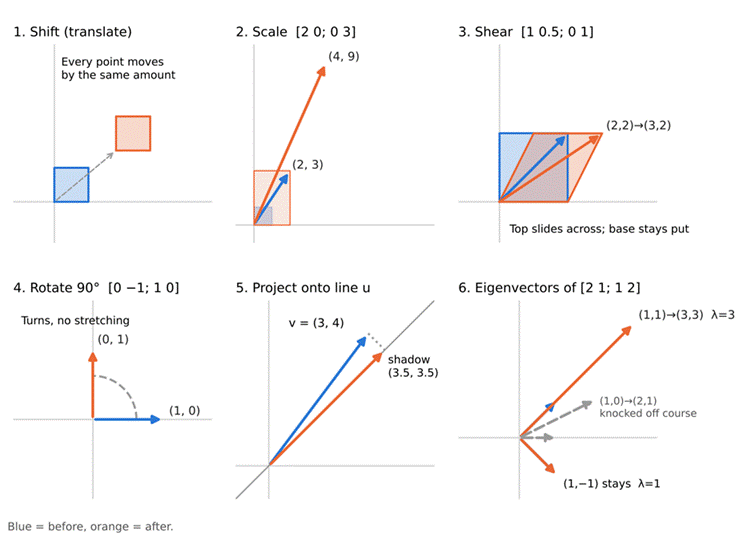
6.1 Shift (translation): change the reference point
(x, y) → (x − a, y − b)
Every point moves by the same amount. The most common use is centring: measuring each item against the average instead of against zero. A house becomes “+200 sq ft and 5 years newer than average” rather than “2,000 sq ft and 20 years old”.
This makes the model’s starting point meaningful (“the price of a typical house”) instead of an abstract “price of a house with zero floor area”. Technically, a shift is not a matrix multiplication (a matrix always leaves zero where it is), so models handle it with an extra “always 1” column, called the bias term in AI.
6.2 Scale: change the units or the importance
[ sₓ 0 ; 0 s_y ] e.g. [ 2 0 ; 0 3 ] turns (2, 3) into (4, 9)
Each axis is stretched or shrunk by its own factor.
- Changing units: square feet to square metres, pounds to dollars. The model’s weights adjust automatically and predictions do not change.
- Standardising: dividing each feature by its typical spread so that, for example, floor area (thousands) does not swamp age (tens). Essential before methods that compare features, such as PCA and clustering.
Note: scaling keeps direction only when every axis is scaled by the same amount. Unequal scaling, like the example above, changes the shape of the data, which is exactly why getting it right matters.
6.3 Shear: adjust one feature for another
[ 1 k ; 0 1 ] e.g. k = 0.5 turns (2, 2) into (3, 2)
One coordinate slides in proportion to the other, like pushing the top of a deck of cards sideways. In data terms it means adjusting one feature for another, e.g. “is this house older than you would expect for its size?” This removes the overlap between two features so the model does not double count.
6.4 Rotation: look from a better angle
[ cos θ −sin θ ; sin θ cos θ ] e.g. θ = 90° turns (1, 0) into (0, 1)
The whole picture turns around the origin. Sin and cos are used because they turn without stretching (cos² + sin² = 1), so distances, and therefore information, are preserved.
Why rotate data? Features often overlap: bigger houses tend to be newer, so “size” and “age” tell much the same story. Rotating the axes so one lines up with that shared pattern turns two tangled features into one clean feature (e.g. “modern and spacious”) plus a small leftover. It is like walking around a sculpture until you find the angle where its shape is clearest.
6.5 Projection: the shadow on what matters
Proj_u(v) = (v · u ÷ u · u) × u e.g. (3, 4) onto u = (1, 1) gives (3.5, 3.5)
A projection is the shadow a vector casts onto a line or plane. It keeps the part pointing along the line and throws away the rest. Two important uses:
- Dimension reduction: after rotating, project onto the important axis and drop the leftover. Two features become one with little information lost. A self-driving car does something similar when it projects 3D sensor points onto the road surface.
- Regression itself is a projection. The model can only produce predictions built from its features; think of that as a flat floor. Its predictions are the shadow of the real outcomes on that floor, and the errors are the perpendicular gap. “Least squares” is simply the shortest drop to the floor, and R² is how much of reality lands in the shadow.
In one line: transformations tidy the data (shift, scale), untangle overlapping features (shear, rotate), and keep only what matters (project).
7. Eigenvectors and Eigenvalues: the Natural Directions in Data
When a matrix transforms vectors, most of them get knocked off course: they end up pointing in a new direction. But a few special directions only get stretched or shrunk, never turned. Those are the eigenvectors, and the amount of stretch is the eigenvalue.
A v = λ v “apply A to v and you get the same v back, just λ times longer”
A simple example
Take the matrix A = [ 2 1 ; 1 2 ] and test three directions:
| Direction v | A × v | What happened |
| (1, 0) | (2, 1) | Knocked off course: not an eigenvector |
| (1, 1) | (3, 3) = 3 × (1, 1) | Same direction, stretched 3×: eigenvector, eigenvalue 3 |
| (1, −1) | (1, −1) = 1 × (1, −1) | Same direction, unchanged: eigenvector, eigenvalue 1 |
Why this matters in ML: Principal Component Analysis (PCA)
If A describes how features vary together (a covariance matrix), then:
- Eigenvectors are the natural directions along which the data is spread out. They are the “best angle” that rotation (6.4) was looking for, found automatically.
- Eigenvalues say how much spread lies in each direction. In the example, 3 ÷ (3 + 1) = 75% of the variation lies along (1, 1) and 25% along (1, −1).
- Keep the directions with big eigenvalues and drop the rest. This is PCA: dozens of overlapping features can be reduced to a handful of strong, independent ones, such as “overall spend” and “electronics vs clothing preference” for customer segmentation.
Another famous example: Google’s PageRank
Google’s original search ranking treated the web as a matrix of links: a page is important if important pages link to it. That circular definition is solved by an eigenvector. Imagine three pages: A links to B and C, B links to C, and C links to A. Someone clicking links at random forever would spend:
| Page A | Page B | Page C |
| 40% of their time | 20% of their time | 40% of their time |
Those shares, (0.4, 0.2, 0.4), are the eigenvector of the link matrix with eigenvalue 1: applying the links again leaves them unchanged. A and C rank highest. Google did the same calculation for billions of pages.
In one line: eigenvectors find the few underlying patterns that really drive the data; eigenvalues say how much each one matters.
8. What Can Go Wrong
- Overlapping features (multicollinearity). When features tell the same story (size, bedrooms, bathrooms), the model can still predict well, but the individual weights become unreliable. Good at “what is it worth?”, weaker at “which feature is worth what?”. Rotation, shearing and PCA are the fixes.
- Missing features (omitted variables). A model cannot see what it is not given. A house-price model with no “condition” feature will undervalue a renovated house. Always ask: what does the model not know?
- Unrepresentative data. A model trained on the wrong examples gives confidently wrong answers. A model can only be as good as the data it learns from.
- Correlation is not causation. Weights describe patterns in past data, not guaranteed effects of changing something.
- Going beyond the data. Predictions far outside the range of the training examples are unreliable.
- No sense-check. Model outputs should always be compared with expert judgement and other evidence before decisions are made.
9. The Whole Story in One Table
| Step | What it does | Business question it answers |
| Vector | Describes one item as numbers | What do we know about this case? |
| Matrix | Holds all the items in one table | What examples can we learn from? |
| Dot product | Facts × weights, added up | What does the model predict for this case? |
| Regression | Learns the weights from past data | What drives the outcome, and by how much? |
| R², F-test, p-values | Measure fit and confidence | Is the pattern real? How wrong could we be? |
| Shift, scale | Put data on a fair, common footing | Are we comparing like with like? |
| Shear, rotate | Untangle overlapping features | Which drivers are really separate? |
| Project | Keep what matters, drop the noise | What is the simplest useful view? |
| Eigenvectors / values | Find the natural directions and their importance | What are the few patterns that really matter? |
For managers: “We describe each case as a list of numbers, learn a recipe from past examples, check the recipe is real and how uncertain it is, tidy and simplify the data so the model sees clearly, and use eigenvectors to find the handful of patterns that matter most. The maths is consistent and explainable, but the model only knows what its data tells it.”
Glossary
| Term | Plain English |
| Vector | A list of numbers describing one thing |
| Matrix | A table of numbers; also a rule that transforms vectors |
| Feature | One fact in a vector (e.g. floor area) |
| Dot product | Multiply matching numbers and add them up |
| Cosine similarity | How closely two vectors point the same way, ignoring size |
| Dependent variable | The outcome being predicted |
| Independent variable | A fact used to make the prediction |
| Weight / parameter | How much a feature contributes to the prediction |
| Least squares | Choosing weights to make the squared errors as small as possible |
| R² | Share of the variation the model explains |
| p-value | Chance of seeing this pattern if there were really no relationship |
| Shift / centring | Measure against a reference point, usually the average |
| Scaling / standardising | Change units or put features on a common scale |
| Shear | Adjust one feature in proportion to another |
| Rotation | Turn the axes without stretching (uses sin and cos) |
| Projection | The shadow of a vector on a line or plane |
| Eigenvector | A direction a matrix only stretches, never turns |
| Eigenvalue | How much an eigenvector is stretched; in PCA, how much variation lies in that direction |
| PCA | Principal Component Analysis: find the main directions in data and keep the important ones |
| Multicollinearity | Features that overlap and tell the same story |